Themen
-
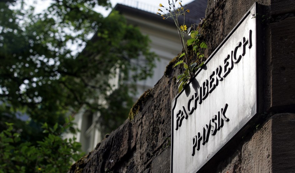
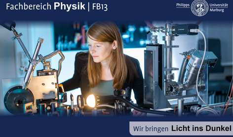
Fachbereich
Von Denis Papin über Alfred Wegener bis Otto Hahn reicht die Liste der Berühmtheiten, die in Marburg Physik studierten und lehrten. Heute gehört Marburg zum Beispiel in der Halbleiterphysik international zu den hervorragenden Forschungsstandorten. Klein aber fein ist der Fachbereich mit seinen etwa 500 Studierenden. -

Studium
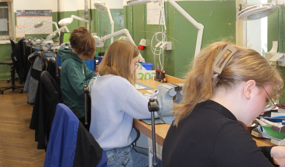
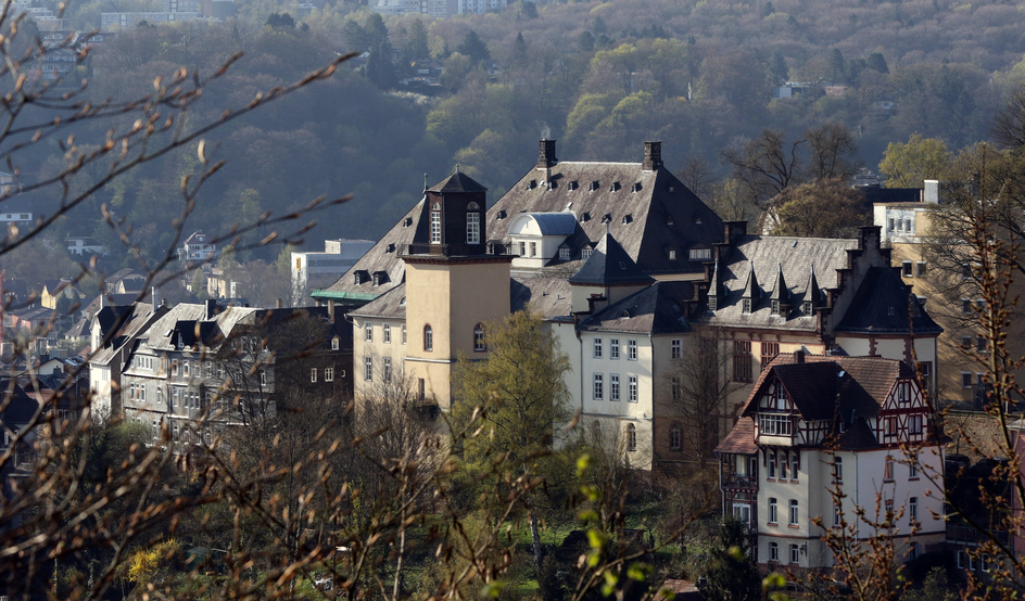
Der Fachbereich Physik mit seinen Campus am Schlossberg und seinen Arbeitsgruppen und Forschungszentren bietet den Studierenden vielfältige Möglichkeiten Physik zu lernen und an vorderster Front zu forschen. -

Forschung
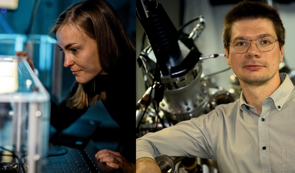
Die Arbeitsgruppen des Fachbereichs sind in vielfältige nationale und internationale Forschungsverbünde und -projekte integriert. Schwerpunkte sind die Halbleiter-, Oberflächen- und Biophysik, sowie die Physik komplexer und chaotischer Systeme. -
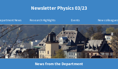
News
Veranstaltungen
-
Fachbereich
Von Denis Papin über Alfred Wegener bis Otto Hahn reicht die Liste der Berühmtheiten, die in Marburg Physik studierten und lehrten. Heute gehört Marburg zum Beispiel in der Halbleiterphysik international zu den hervorragenden Forschungsstandorten. Klein aber fein ist der Fachbereich mit seinen etwa 500 Studierenden. -
Studium
Der Fachbereich Physik mit seinen Campus am Schlossberg und seinen Arbeitsgruppen und Forschungszentren bietet den Studierenden vielfältige Möglichkeiten Physik zu lernen und an vorderster Front zu forschen. -
Forschung
Die Arbeitsgruppen des Fachbereichs sind in vielfältige nationale und internationale Forschungsverbünde und -projekte integriert. Schwerpunkte sind die Halbleiter-, Oberflächen- und Biophysik, sowie die Physik komplexer und chaotischer Systeme. -
News
Veranstaltungen